|
OpenCV 4.12.0
开源计算机视觉
|
加载中...
搜索中...
无匹配项
|
OpenCV 4.12.0
开源计算机视觉
|
OpenCV(开源计算机视觉)是一个流行的计算机视觉库,由英特尔(Intel)于1999年启动。这个跨平台库专注于实时图像处理,并包含最新计算机视觉算法的无专利实现。2008年,Willow Garage接手了支持工作,OpenCV 2.3.1现在提供了C、C++、Python和Android的编程接口。OpenCV在BSD许可下发布,因此它在学术项目和商业产品中都有使用。
OpenCV 2.4现在附带了全新的FaceRecognizer类,用于人脸识别,因此您可以立即开始人脸识别的实验。本文档是我在研究人脸识别时所希望得到的指南。它将向您展示如何在OpenCV中使用FaceRecognizer进行人脸识别(包含完整的源代码列表),并介绍其背后的算法。我还会展示如何创建许多出版物中常见的可视化效果,因为很多人都提出了要求。
目前可用的算法有
您无需从本页复制粘贴源代码示例,因为它们已随本文档一起提供在 src 文件夹中。如果您在构建 OpenCV 时启用了示例,那么很可能它们已经被编译了!尽管对于高级用户来说可能很有趣,但我决定省略实现细节,因为我担心它们会使新用户感到困惑。
本文档中的所有代码均在BSD 许可下发布,因此您可以随意将其用于您的项目。
人脸识别对人类来说是一项简单的任务。[278]中的实验表明,即使是一到三天大的婴儿也能够区分已知的人脸。那么,对于计算机来说,这有多难呢?事实证明,我们对人类识别的了解甚少。人脸识别的成功是否使用了内部特征(眼睛、鼻子、嘴巴)或外部特征(头部形状、发际线)?我们如何分析图像,大脑又如何对其进行编码?大卫·休贝尔(David Hubel)和托尔斯顿·维瑟尔(Torsten Wiesel)的研究表明,我们的大脑具有专门的神经细胞,对场景中的特定局部特征(如线条、边缘、角度或运动)做出反应。由于我们不将世界视为零散的碎片,我们的视觉皮层必须以某种方式将不同来源的信息组合成有用的模式。自动人脸识别就是从图像中提取这些有意义的特征,将它们放入有用的表示形式中,并对其进行某种分类。
基于人脸几何特征的人脸识别可能是最直观的人脸识别方法之一。[144]中描述了最早的自动化人脸识别系统之一:使用标记点(眼睛、耳朵、鼻子等的位置)来构建特征向量(点之间的距离、它们之间的角度等)。识别通过计算探查图像和参考图像的特征向量之间的欧几里得距离来执行。这种方法本质上对光照变化具有鲁棒性,但有一个巨大的缺点:即使使用最先进的算法,标记点的精确注册也相当复杂。最近关于几何人脸识别的一些工作是在[44]中进行的。该研究使用了22维特征向量,并在大型数据集上进行的实验表明,单独的几何特征可能不足以用于人脸识别。
[279]中描述的特征脸方法采用了人脸识别的整体方法:人脸图像是高维图像空间中的一个点,通过找到一个较低维的表示,分类变得容易。较低维子空间通过主成分分析(Principal Component Analysis,PCA)找到,该分析识别出具有最大方差的轴。虽然这种转换从重建的角度来看是最佳的,但它没有考虑任何类别标签。想象一下,方差是由外部来源(比如光照)产生的。具有最大方差的轴不一定包含任何判别信息,因此分类变得不可能。因此,在[24]中,将带有线性判别分析(Linear Discriminant Analysis)的类别特定投影应用于人脸识别。其基本思想是最小化类别内部的方差,同时最大化类别之间的方差。
最近出现了各种局部特征提取方法。为了避免输入数据的高维度,仅描述图像的局部区域,提取的特征(希望)对部分遮挡、光照和少量样本更具鲁棒性。用于局部特征提取的算法有Gabor小波([301])、离散余弦变换([192])和局部二值模式([3])。在应用局部特征提取时,如何最好地保留空间信息仍然是一个开放的研究问题,因为空间信息是潜在的有用信息。
首先,让我们获取一些数据进行实验。我这里不想做玩具示例。我们正在进行人脸识别,所以你需要一些人脸图像!你可以创建自己的数据集,或者从现有的人脸数据库中选择一个。http://face-rec.org/databases/提供了最新的概览。三个有趣的数据集是(部分描述引用自http://face-rec.org):
耶鲁人脸数据库 A,也称为Yalefaces。AT&T人脸数据库适合初步测试,但它是一个相当容易的数据库。特征脸方法在该数据库上已经达到了97%的识别率,因此使用其他算法您不会看到显著的改进。耶鲁人脸数据库A(也称为Yalefaces)更适合初步实验,因为识别问题更难。该数据库包含15个人(14名男性,1名女性),每个人有11张灰度图像,大小为\(320 \times 243\)像素。光照条件(中心光、左侧光、右侧光)、面部表情(开心、正常、悲伤、困倦、惊讶、眨眼)和眼镜(戴眼镜、不戴眼镜)都有变化。
原始图像未经过裁剪和对齐。请查看附录中的Python脚本,它可以为您完成这项工作。
一旦我们获取了数据,就需要将其读入程序。在演示应用程序中,我决定从一个非常简单的CSV文件中读取图像。为什么?因为这是我能想到的最简单的平台无关方法。但是,如果您知道更简单的解决方案,请告诉我。基本上,所有CSV文件都需要包含的行都由文件名、分号“;”和标签(整数)组成,像这样:
让我们分析一下这一行。/path/to/image.ext是图像的路径,如果您在Windows中,可能像这样:C:/faces/person0/image0.jpg。然后是分隔符“;”,最后我们将标签0分配给该图像。将标签视为此图像所属的主体(人物),因此相同的主体(人物)应具有相同的标签。
从AT&T人脸数据库下载AT&T人脸数据库,并从at.txt下载相应的CSV文件,其内容如下(文件当然没有...):
假设我已经将文件提取到 D:/data/at,并将CSV文件下载到 D:/data/at.txt。那么你只需将 `./` 替换为 `D:/data/` 即可。您可以在您选择的编辑器中完成此操作,任何足够高级的编辑器都可以做到这一点。一旦您有了包含有效文件名和标签的CSV文件,就可以通过将CSV文件的路径作为参数传递来运行任何演示程序:
请参阅创建CSV文件了解创建CSV文件的详细信息。
我们所得到的图像表示存在的问题是其高维度。二维的\(p \times q\)灰度图像构成一个\(m = pq\)维的向量空间,因此一个\(100 \times 100\)像素的图像已经位于一个\(10,000\)维的图像空间中。问题是:所有维度对我们都同样有用吗?只有数据存在方差时我们才能做出决策,因此我们正在寻找那些能解释大部分信息的成分。主成分分析(PCA)由卡尔·皮尔逊(Karl Pearson)(1901年)和哈罗德·霍特林(Harold Hotelling)(1933年)独立提出,旨在将一组可能相关的变量转换为一组较小的、不相关的变量。其思想是,高维数据集通常由相关变量描述,因此只有少数有意义的维度解释了大部分信息。PCA方法找到数据中方差最大的方向,这些方向被称为主成分。
设 \(X = \{ x_{1}, x_{2}, \ldots, x_{n} \}\) 是具有观测值 \(x_i \in R^{d}\) 的随机向量。
计算均值 \(\mu\)
\[\mu = \frac{1}{n} \sum_{i=1}^{n} x_{i}\]
计算协方差矩阵 S
\[S = \frac{1}{n} \sum_{i=1}^{n} (x_{i} - \mu) (x_{i} - \mu)^{T}`\]
计算 \(S\) 的特征值 \(\lambda_{i}\) 和特征向量 \(v_{i}\)
\[S v_{i} = \lambda_{i} v_{i}, i=1,2,\ldots,n\]
观测向量 \(x\) 的 \(k\) 个主成分由下式给出
\[y = W^{T} (x - \mu)\]
其中 \(W = (v_{1}, v_{2}, \ldots, v_{k})\)。
从PCA基的重构由下式给出
\[x = W y + \mu\]
其中 \(W = (v_{1}, v_{2}, \ldots, v_{k})\)。
特征脸方法通过以下步骤进行人脸识别:
仍然有一个问题需要解决。假设我们有\(400\)张大小为\(100 \times 100\)像素的图像。主成分分析求解协方差矩阵\(S = X X^{T}\),在我们的例子中,\({size}(X) = 10000 \times 400\)。你最终会得到一个\(10000 \times 10000\)的矩阵,大约\(0.8 GB\)。解决这个问题是不可行的,所以我们需要应用一个技巧。从你的线性代数课程中你知道,一个\(M \times N\)矩阵,当\(M > N\)时,只能有\(N - 1\)个非零特征值。因此,可以改为进行大小为\(N \times N\)的特征值分解\(S = X^{T} X\)
\[X^{T} X v_{i} = \lambda_{i} v{i}\]
并通过数据矩阵的左乘得到\(S = X X^{T}\)的原始特征向量
\[X X^{T} (X v_{i}) = \lambda_{i} (X v_{i})\]
得到的特征向量是正交的,为了获得标准正交特征向量,需要将它们归一化到单位长度。我不想把这变成一篇论文,所以请查阅[77]以获取这些方程的推导和证明。
对于第一个源代码示例,我将和您一起过一遍。我首先会给出完整的源代码列表,然后我们将详细查看其中最重要的几行。请注意:每个源代码列表都已详细注释,因此您应该能够轻松理解。
此演示应用程序的源代码也随本文档提供在 src 文件夹中
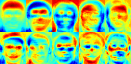
我使用了jet颜色映射,这样您就可以看到灰度值在特定特征脸中的分布情况。您可以看到,特征脸不仅编码了面部特征,还编码了图像中的光照信息(参见特征脸#4中的左侧光,特征脸#5中的右侧光)。
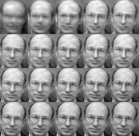
我们已经看到,可以从较低维度的近似值中重建人脸。那么,一个好的重建需要多少个特征脸呢?我将使用\(10,30,\ldots,310\)个特征脸绘制一个子图。
10个特征向量显然不足以进行良好的图像重建,而50个特征向量可能已经足以编码重要的面部特征。对于AT&T人脸数据库,大约300个特征向量就可以获得良好的重建效果。关于成功人脸识别应该选择多少个特征脸,有一些经验法则,但这在很大程度上取决于输入数据。[322]是开始研究这个问题的最佳切入点。
主成分分析(PCA)是特征脸方法的核心,它找到特征的线性组合,使数据中的总方差最大化。虽然这显然是一种强大的数据表示方法,但它没有考虑任何类别,因此在丢弃成分时可能会丢失大量判别信息。想象一下,您的数据中的方差是由外部来源(例如光照)产生的。PCA识别出的成分不一定包含任何判别信息,因此投影后的样本会混杂在一起,导致分类变得不可能(参见http://www.bytefish.de/wiki/pca_lda_with_gnu_octave了解示例)。
线性判别分析执行类别特定的降维,由伟大的统计学家R. A. 费舍尔爵士(Sir R. A. Fisher)发明。他在1936年的论文《多重测量在分类问题中的应用》[93]中成功地将其用于花卉分类。为了找到能够最好地分离类别的特征组合,线性判别分析最大化了类间散度与类内散度之比,而不是最大化总体散度。这个思想很简单:在低维表示中,相同类别应该紧密地聚集在一起,而不同类别则尽可能地相互远离。这一观点也得到了Belhumeur、Hespanha和Kriegman的认可,因此他们在[24]中将判别分析应用于人脸识别。
设 \(X\) 是一个随机向量,其样本从 \(c\) 个类别中抽取
\[\begin{align*} X & = & \{X_1,X_2,\ldots,X_c\} \\ X_i & = & \{x_1, x_2, \ldots, x_n\} \end{align*}\]
散度矩阵 \(S_{B}\) 和 S_{W} 的计算方式如下
\[\begin{align*} S_{B} & = & \sum_{i=1}^{c} N_{i} (\mu_i - \mu)(\mu_i - \mu)^{T} \\ S_{W} & = & \sum_{i=1}^{c} \sum_{x_{j} \in X_{i}} (x_j - \mu_i)(x_j - \mu_i)^{T} \end{align*}\]
,其中 \(\mu\) 是总均值
\[\mu = \frac{1}{N} \sum_{i=1}^{N} x_i\]
而 \(\mu_i\) 是类别 \(i \in \{1,\ldots,c\}\) 的均值
\[\mu_i = \frac{1}{|X_i|} \sum_{x_j \in X_i} x_j\]
费舍尔的经典算法现在寻找一个投影 \(W\),它最大化类别可分离性准则
\[W_{opt} = \operatorname{arg\,max}_{W} \frac{|W^T S_B W|}{|W^T S_W W|}\]
遵循[24],此优化问题的解通过求解广义特征值问题给出
\[\begin{align*} S_{B} v_{i} & = & \lambda_{i} S_w v_{i} \nonumber \\ S_{W}^{-1} S_{B} v_{i} & = & \lambda_{i} v_{i} \end{align*}\]
还有一个问题需要解决:\(S_{W}\)的秩最多为\((N-c)\),其中\(N\)是样本数,\(c\)是类别数。在模式识别问题中,样本数\(N\)几乎总是小于输入数据的维度(像素数),因此散度矩阵\(S_{W}\)会变得奇异(参见[226])。在[24]中,这个问题通过对数据执行主成分分析并将样本投影到\((N-c)\)维空间来解决。然后对降维后的数据执行线性判别分析,因为此时\(S_{W}\)不再奇异。
优化问题可以改写为
\[\begin{align*} W_{pca} & = & \operatorname{arg\,max}_{W} |W^T S_T W| \\ W_{fld} & = & \operatorname{arg\,max}_{W} \frac{|W^T W_{pca}^T S_{B} W_{pca} W|}{|W^T W_{pca}^T S_{W} W_{pca} W|} \end{align*}\]
将样本投影到\((c-1)\)维空间的变换矩阵\(W\)由下式给出
\[W = W_{fld}^{T} W_{pca}^{T}\]
此演示应用程序的源代码也随本文档提供在 src 文件夹中
对于这个例子,我将使用耶鲁人脸数据库A,仅仅因为图表更好看。每个费舍尔脸与原始图像的长度相同,因此可以作为图像显示。演示显示(或保存)了前16个费舍尔脸(最多)。
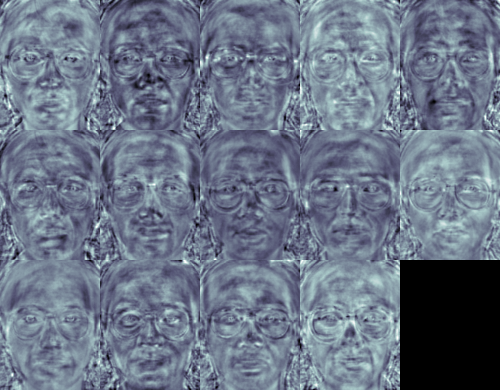
费舍尔脸方法学习类别特定的变换矩阵,因此它们不像特征脸方法那样明显地捕捉光照。判别分析反而会找到区分人脸的特征。值得一提的是,费舍尔脸的性能也严重依赖于输入数据。实际上:如果您仅针对光照良好的图片学习费舍尔脸,并尝试在光照不良的场景中识别人脸,那么该方法很可能会找到错误的组件(仅仅因为这些特征在光照不良的图像上可能不占主导地位)。这在某种程度上是合乎逻辑的,因为该方法没有机会学习光照。
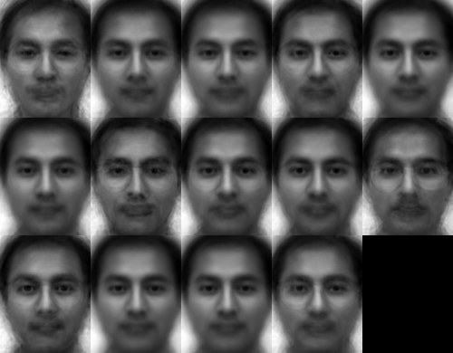
费舍尔脸允许重构投影图像,就像特征脸一样。但是,由于我们只识别了区分不同主体的特征,所以不能期望原始图像的完美重构。对于费舍尔脸方法,我们将样本图像投影到每个费舍尔脸上。这样您将有一个很好的可视化效果,显示每个费舍尔脸描述了哪些特征。
这些差异对于人眼来说可能很微妙,但您应该能够看到一些不同之处。
特征脸和费舍尔脸在人脸识别中采取了一种整体方法。你将数据视为高维图像空间中的一个向量。我们都知道高维度是不好的,因此会识别一个较低维的子空间,其中(可能)保留了有用的信息。特征脸方法最大化总散度,如果方差是由外部来源产生的,这可能会导致问题,因为在所有类别上具有最大方差的组件不一定对分类有用(参见http://www.bytefish.de/wiki/pca_lda_with_gnu_octave)。因此,为了保留一些判别信息,我们应用了线性判别分析并按照费舍尔脸方法中描述的进行了优化。费舍尔脸方法效果很好……至少对于我们模型中假定的受限场景而言。
现实生活并不完美。你根本无法保证图像中有完美的光照设置,或者一个人有10张不同的图像。那么,如果每个人只有一张图像呢?我们对子空间的协方差估计可能会严重错误,识别结果也会如此。还记得特征脸方法在AT&T人脸数据库上的识别率达到96%吗?我们实际需要多少张图像才能获得如此有用的估计?以下是特征脸和费舍尔脸方法在AT&T人脸数据库(一个相当简单的图像数据库)上的Rank-1识别率:
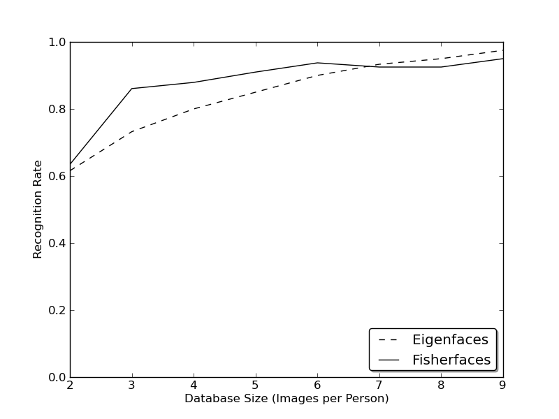
因此,为了获得良好的识别率,您需要每个人至少有8(±1)张图像,而费舍尔脸方法在这方面并没有真正帮助。上述实验是使用facerec框架在https://github.com/bytefish/facerec上进行的10折交叉验证结果。这不是一篇论文,所以我不会用深入的数学分析来支持这些数据。关于小训练数据集下这两种方法的详细分析,请查阅[186]。
因此,一些研究集中于从图像中提取局部特征。其思想是,不将整个图像视为高维向量,而是只描述对象的局部特征。以这种方式提取的特征将隐式地具有低维度。这是一个不错的想法!但是您很快就会发现,我们得到的图像表示不仅受光照变化的影响。考虑图像中的缩放、平移或旋转等因素——您的局部描述至少要对这些因素有一定的鲁棒性。就像SIFT一样,局部二值模式方法论起源于二维纹理分析。局部二值模式的基本思想是通过将每个像素与其邻域进行比较来概括图像中的局部结构。将一个像素作为中心,并将其邻居与其进行阈值比较。如果中心像素的强度大于或等于其邻居,则标记为1,否则标记为0。您最终将为每个像素得到一个二进制数,就像这样:

LBP算子更正式的描述可以给出为
\[LBP(x_c, y_c) = \sum_{p=0}^{P-1} 2^p s(i_p - i_c)\]
,其中 \((x_c, y_c)\) 是强度为 \(i_c\) 的中心像素;而 \(i_n\) 是邻居像素的强度。\(s\) 是符号函数,定义为
\[\begin{equation} s(x) = \begin{cases} 1 & \text{if \(x \geq 0\)}\\ 0 & \text{else} \end{cases} \end{equation}\]
这种描述使您能够捕捉图像中非常细微的细节。事实上,作者在纹理分类方面能够与最先进的结果相媲美。该算子发表后不久,人们注意到固定邻域无法编码尺度不同的细节。因此,该算子在[3]中被扩展为使用可变邻域。其思想是在一个可变半径的圆上对齐任意数量的邻居,从而能够捕捉以下邻域:
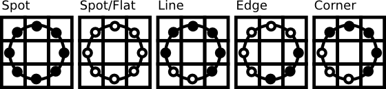
对于给定的点 \((x_c,y_c)\),邻居 \((x_p,y_p), p \in P\) 的位置可以通过以下公式计算:
\[\begin{align*} x_{p} & = & x_c + R \cos({\frac{2\pi p}{P}})\\ y_{p} & = & y_c - R \sin({\frac{2\pi p}{P}}) \end{align*}\]
其中 \(R\) 是圆的半径,\(P\) 是采样点的数量。
该算子是原始LBP码的扩展,因此有时被称为扩展LBP(或圆形LBP)。如果圆上点的坐标与图像坐标不对应,则该点将被插值。计算机科学有许多巧妙的插值方案,OpenCV实现的是双线性插值。
\[\begin{align*} f(x,y) \approx \begin{bmatrix} 1-x & x \end{bmatrix} \begin{bmatrix} f(0,0) & f(0,1) \\ f(1,0) & f(1,1) \end{bmatrix} \begin{bmatrix} 1-y \\ y \end{bmatrix}. \end{align*}\]
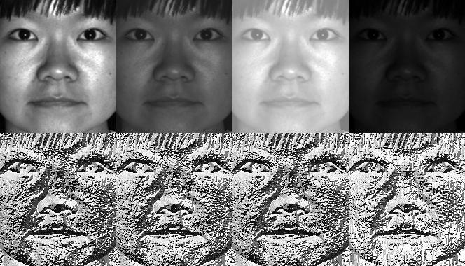
根据定义,LBP算子对单调灰度变换具有鲁棒性。我们可以通过观察人工修改图像的LBP图像轻松验证这一点(这样您就能看到LBP图像的样子!)。
那么剩下的就是如何将空间信息整合到人脸识别模型中。Ahonen等人[3]提出的表示方法是将LBP图像划分为\(m\)个局部区域,并从每个区域提取一个直方图。然后通过连接这些局部直方图(而非合并它们)获得空间增强的特征向量。这些直方图被称为局部二值模式直方图。
此演示应用程序的源代码也随本文档提供在 src 文件夹中
您已经学会了如何在实际应用程序中使用新的 FaceRecognizer。阅读本文档后,您也了解了算法的工作原理,现在是时候您自己尝试这些可用算法了。使用它们,改进它们,并让 OpenCV 社区参与进来!
如果没有使用AT&T人脸数据库和耶鲁人脸数据库A/B中的人脸图像的慷慨许可,本文档将无法完成。
重要提示:使用这些图像时,请注明“AT&T实验室,剑桥”。
人脸数据库,前身为ORL人脸数据库,包含1992年4月至1994年4月期间拍摄的一组人脸图像。该数据库是在与剑桥大学工程系语音、视觉和机器人小组合作进行的人脸识别项目中使用的。
该数据库包含40个不同主体的每人十张不同图像。对于某些主体,图像在不同时间拍摄,光照、面部表情(睁眼/闭眼、微笑/不微笑)和面部细节(戴眼镜/不戴眼镜)各不相同。所有图像均在黑暗均匀的背景下拍摄,主体处于直立、正面位置(允许一定的侧向移动)。
文件为PGM格式。每张图像大小为92x112像素,每个像素有256个灰度级别。图像组织在40个目录中(每个主体一个),目录名称形式为sX,其中X表示主体编号(1到40之间)。在每个目录中,都有该主体的十张不同图像,图像名称形式为Y.pgm,其中Y是该主体的图像编号(1到10之间)。
数据库副本可从以下地址获取:http://www.cl.cam.ac.uk/research/dtg/attarchive/pub/data/att_faces.zip。
经作者许可,我被允许展示少量图像(例如主体1及其所有变体),以及来自耶鲁人脸数据库A或耶鲁人脸数据库B的所有图像,例如费舍尔脸和特征脸。
耶鲁人脸数据库A(大小6.4MB)包含15个人的165张GIF格式的灰度图像。每个主体有11张图像,对应不同的面部表情或配置:中心光照、戴眼镜、高兴、左侧光照、不戴眼镜、正常、右侧光照、悲伤、困倦、惊讶和眨眼。(来源:http://cvc.yale.edu/projects/yalefaces/yalefaces.html)
经作者许可,我被允许展示少量图像(例如主体1及其所有变体),以及来自耶鲁人脸数据库A或耶鲁人脸数据库B的所有图像,例如费舍尔脸和特征脸。
扩展耶鲁人脸数据库B包含28个主体在9种姿态和64种光照条件下的16128张图像。该数据库的数据格式与耶鲁人脸数据库B相同。有关数据格式的更详细信息,请参阅耶鲁人脸数据库B的主页(或本页的副本)。
您可以自由地将扩展耶鲁人脸数据库B用于研究目的。所有使用此数据库的出版物都应注明“Exteded Yale Face Database B”的使用,并引用Athinodoros Georghiades、Peter Belhumeur和David Kriegman的论文,“From Few to Many: Illumination Cone Models for Face Recognition under Variable Lighting and Pose”,PAMI,2001年,[bibtex]。
扩展数据库(与原始的10个主体的耶鲁人脸数据库B相对)首次由Kuang-Chih Lee、Jeffrey Ho和David Kriegman在2005年5月PAMI发表的“Acquiring Linear Subspaces for Face Recognition under Variable Lighting”中报告,[pdf]。实验中使用的所有测试图像数据均经过手动对齐、裁剪,然后重新调整大小为168x192图像。如果您发布裁剪图像的实验结果,也请引用PAMI2005论文。(来源:http://vision.ucsd.edu/~leekc/ExtYaleDatabase/ExtYaleB.html)
您肯定不想手动创建CSV文件。我已经为您准备了一个小型Python脚本 create_csv.py(您可以在本教程附带的 src/create_csv.py 中找到它),它会自动为您创建一个CSV文件。如果您的图像按以下层次结构排列(/basepath/<subject>/<image.ext>):
那么只需调用 create_csv.py at,其中 'at' 是文件夹的基路径,就像这样,你就可以保存输出了:
如果您找不到脚本,请看这里:
#!/usr/bin/env python

import sys
import os.path

# This is a tiny script to help you creating a CSV file from a face
# database with a similar hierarchie:
#
#  philipp@mango:~/facerec/data/at$ tree
#  .
#  |-- README
#  |-- s1
#  |   |-- 1.pgm
#  |   |-- ...
#  |   |-- 10.pgm
#  |-- s2
#  |   |-- 1.pgm
#  |   |-- ...
#  |   |-- 10.pgm
#  ...
#  |-- s40
#  |   |-- 1.pgm
#  |   |-- ...
#  |   |-- 10.pgm
#

if __name__ == "__main__":

    if len(sys.argv) != 2:
        print "usage: create_csv <base_path>"
        sys.exit(1)

    BASE_PATH=sys.argv[1]
    SEPARATOR=";"

    label = 0
    for dirname, dirnames, filenames in os.walk(BASE_PATH):
        for subdirname in dirnames:
            subject_path = os.path.join(dirname, subdirname)
            for filename in os.listdir(subject_path):
                abs_path = "%s/%s" % (subject_path, filename)
                print "%s%s%d" % (abs_path, SEPARATOR, label)
            label = label + 1
图像数据的精确对齐在情绪检测等任务中尤为重要,因为您需要尽可能多的细节。相信我……您不想手动完成这项工作。所以我为您准备了一个小巧的Python脚本。代码使用起来非常简单。要缩放、旋转和裁剪人脸图像,您只需调用 CropFace(image, eye_left, eye_right, offset_pct, dest_sz),其中:
如果您对所有图像都使用相同的offset_pct和dest_sz,那么它们都会以眼睛为基准进行对齐。
#!/usr/bin/env python
# Software License Agreement (BSD License)
#
# Copyright (c) 2012, Philipp Wagner
# All rights reserved.
#
# Redistribution and use in source and binary forms, with or without
# modification, are permitted provided that the following conditions
# are met:
#
#  * Redistributions of source code must retain the above copyright
#    notice, this list of conditions and the following disclaimer.
#  * Redistributions in binary form must reproduce the above
#    copyright notice, this list of conditions and the following
#    disclaimer in the documentation and/or other materials provided
#    with the distribution.
#  * Neither the name of the author nor the names of its
#    contributors may be used to endorse or promote products derived
#    from this software without specific prior written permission.
#
# THIS SOFTWARE IS PROVIDED BY THE COPYRIGHT HOLDERS AND CONTRIBUTORS
# "AS IS" AND ANY EXPRESS OR IMPLIED WARRANTIES, INCLUDING, BUT NOT
# LIMITED TO, THE IMPLIED WARRANTIES OF MERCHANTABILITY AND FITNESS
# FOR A PARTICULAR PURPOSE ARE DISCLAIMED. IN NO EVENT SHALL THE
# COPYRIGHT OWNER OR CONTRIBUTORS BE LIABLE FOR ANY DIRECT, INDIRECT,
# INCIDENTAL, SPECIAL, EXEMPLARY, OR CONSEQUENTIAL DAMAGES (INCLUDING,
# BUT NOT LIMITED TO, PROCUREMENT OF SUBSTITUTE GOODS OR SERVICES;
# LOSS OF USE, DATA, OR PROFITS; OR BUSINESS INTERRUPTION) HOWEVER
# CAUSED AND ON ANY THEORY OF LIABILITY, WHETHER IN CONTRACT, STRICT
# LIABILITY, OR TORT (INCLUDING NEGLIGENCE OR OTHERWISE) ARISING IN
# ANY WAY OUT OF THE USE OF THIS SOFTWARE, EVEN IF ADVISED OF THE
# POSSIBILITY OF SUCH DAMAGE.

import sys, math, Image

def Distance(p1,p2):
  dx = p2[0] - p1[0]
  dy = p2[1] - p1[1]
  return math.sqrt(dx*dx+dy*dy)

def ScaleRotateTranslate(image, angle, center = None, new_center = None, scale = None, resample=Image.BICUBIC):
  if (scale is None) and (center is None):
    return image.rotate(angle=angle, resample=resample)
  nx,ny = x,y = center
  sx=sy=1.0
  if new_center:
    (nx,ny) = new_center
  if scale:
    (sx,sy) = (scale, scale)
  cosine = math.cos(angle)
  sine = math.sin(angle)
  a = cosine/sx
  b = sine/sx
  c = x-nx*a-ny*b
  d = -sine/sy
  e = cosine/sy
  f = y-nx*d-ny*e
  return image.transform(image.size, Image.AFFINE, (a,b,c,d,e,f), resample=resample)

def CropFace(image, eye_left=(0,0), eye_right=(0,0), offset_pct=(0.2,0.2), dest_sz = (70,70)):
  # calculate offsets in original image
  offset_h = math.floor(float(offset_pct[0])*dest_sz[0])
  offset_v = math.floor(float(offset_pct[1])*dest_sz[1])
  # get the direction
  eye_direction = (eye_right[0] - eye_left[0], eye_right[1] - eye_left[1])
  # calc rotation angle in radians
  rotation = -math.atan2(float(eye_direction[1]),float(eye_direction[0]))
  # distance between them
  dist = Distance(eye_left, eye_right)
  # calculate the reference eye-width
  reference = dest_sz[0] - 2.0*offset_h
  # scale factor
  scale = float(dist)/float(reference)
  # rotate original around the left eye
  image = ScaleRotateTranslate(image, center=eye_left, angle=rotation)
  # crop the rotated image
  crop_xy = (eye_left[0] - scale*offset_h, eye_left[1] - scale*offset_v)
  crop_size = (dest_sz[0]*scale, dest_sz[1]*scale)
  image = image.crop((int(crop_xy[0]), int(crop_xy[1]), int(crop_xy[0]+crop_size[0]), int(crop_xy[1]+crop_size[1])))
  # resize it
  image = image.resize(dest_sz, Image.ANTIALIAS)
  return image

def readFileNames():
    try:
        inFile = open('path_to_created_csv_file.csv')
    except:
        raise IOError('There is no file named path_to_created_csv_file.csv in current directory.')
        return False

    picPath = []
    picIndex = []

    for line in inFile.readlines():
        if line != '':
            fields = line.rstrip().split(';')
            picPath.append(fields[0])
            picIndex.append(int(fields[1]))

    return (picPath, picIndex)


if __name__ == "__main__":
  [images, indexes]=readFileNames()
if not os.path.exists("modified"):
    os.makedirs("modified")
for img in images:
    image =  Image.open(img)
    CropFace(image, eye_left=(252,364), eye_right=(420,366), offset_pct=(0.1,0.1), dest_sz=(200,200)).save("modified/"+img.rstrip().split('/')[1]+"_10_10_200_200.jpg")
    CropFace(image, eye_left=(252,364), eye_right=(420,366), offset_pct=(0.2,0.2), dest_sz=(200,200)).save("modified/"+img.rstrip().split('/')[1]+"_20_20_200_200.jpg")
    CropFace(image, eye_left=(252,364), eye_right=(420,366), offset_pct=(0.3,0.3), dest_sz=(200,200)).save("modified/"+img.rstrip().split('/')[1]+"_30_30_200_200.jpg")
    CropFace(image, eye_left=(252,364), eye_right=(420,366), offset_pct=(0.2,0.2)).save("modified/"+img.rstrip().split('/')[1]+"_20_20_70_70.jpg")
想象一下,我们有一张阿诺德·施瓦辛格的这张照片,它处于公共领域许可之下。左眼的大致(x,y)位置是(252,364),右眼是(420,366)。现在您只需要定义水平偏移量、垂直偏移量以及缩放、旋转和裁剪后人脸的尺寸。
这里有一些示例
| 配置 | 裁剪、缩放、旋转后的人脸 |
|---|---|
| 0.1 (10%), 0.1 (10%), (200,200) |  |
| 0.2 (20%), 0.2 (20%), (200,200) |  |
| 0.3 (30%), 0.3 (30%), (200,200) |  |
| 0.2 (20%), 0.2 (20%), (70,70) |  |
/home/philipp/facerec/data/at/s13/2.pgm;12
/home/philipp/facerec/data/at/s13/7.pgm;12
/home/philipp/facerec/data/at/s13/6.pgm;12
/home/philipp/facerec/data/at/s13/9.pgm;12
/home/philipp/facerec/data/at/s13/5.pgm;12
/home/philipp/facerec/data/at/s13/3.pgm;12
/home/philipp/facerec/data/at/s13/4.pgm;12
/home/philipp/facerec/data/at/s13/10.pgm;12
/home/philipp/facerec/data/at/s13/8.pgm;12
/home/philipp/facerec/data/at/s13/1.pgm;12
/home/philipp/facerec/data/at/s17/2.pgm;16
/home/philipp/facerec/data/at/s17/7.pgm;16
/home/philipp/facerec/data/at/s17/6.pgm;16
/home/philipp/facerec/data/at/s17/9.pgm;16
/home/philipp/facerec/data/at/s17/5.pgm;16
/home/philipp/facerec/data/at/s17/3.pgm;16
/home/philipp/facerec/data/at/s17/4.pgm;16
/home/philipp/facerec/data/at/s17/10.pgm;16
/home/philipp/facerec/data/at/s17/8.pgm;16
/home/philipp/facerec/data/at/s17/1.pgm;16
/home/philipp/facerec/data/at/s32/2.pgm;31
/home/philipp/facerec/data/at/s32/7.pgm;31
/home/philipp/facerec/data/at/s32/6.pgm;31
/home/philipp/facerec/data/at/s32/9.pgm;31
/home/philipp/facerec/data/at/s32/5.pgm;31
/home/philipp/facerec/data/at/s32/3.pgm;31
/home/philipp/facerec/data/at/s32/4.pgm;31
/home/philipp/facerec/data/at/s32/10.pgm;31
/home/philipp/facerec/data/at/s32/8.pgm;31
/home/philipp/facerec/data/at/s32/1.pgm;31
/home/philipp/facerec/data/at/s10/2.pgm;9
/home/philipp/facerec/data/at/s10/7.pgm;9
/home/philipp/facerec/data/at/s10/6.pgm;9
/home/philipp/facerec/data/at/s10/9.pgm;9
/home/philipp/facerec/data/at/s10/5.pgm;9
/home/philipp/facerec/data/at/s10/3.pgm;9
/home/philipp/facerec/data/at/s10/4.pgm;9
/home/philipp/facerec/data/at/s10/10.pgm;9
/home/philipp/facerec/data/at/s10/8.pgm;9
/home/philipp/facerec/data/at/s10/1.pgm;9
/home/philipp/facerec/data/at/s27/2.pgm;26
/home/philipp/facerec/data/at/s27/7.pgm;26
/home/philipp/facerec/data/at/s27/6.pgm;26
/home/philipp/facerec/data/at/s27/9.pgm;26
/home/philipp/facerec/data/at/s27/5.pgm;26
/home/philipp/facerec/data/at/s27/3.pgm;26
/home/philipp/facerec/data/at/s27/4.pgm;26
/home/philipp/facerec/data/at/s27/10.pgm;26
/home/philipp/facerec/data/at/s27/8.pgm;26
/home/philipp/facerec/data/at/s27/1.pgm;26
/home/philipp/facerec/data/at/s5/2.pgm;4
/home/philipp/facerec/data/at/s5/7.pgm;4
/home/philipp/facerec/data/at/s5/6.pgm;4
/home/philipp/facerec/data/at/s5/9.pgm;4
/home/philipp/facerec/data/at/s5/5.pgm;4
/home/philipp/facerec/data/at/s5/3.pgm;4
/home/philipp/facerec/data/at/s5/4.pgm;4
/home/philipp/facerec/data/at/s5/10.pgm;4
/home/philipp/facerec/data/at/s5/8.pgm;4
/home/philipp/facerec/data/at/s5/1.pgm;4
/home/philipp/facerec/data/at/s20/2.pgm;19
/home/philipp/facerec/data/at/s20/7.pgm;19
/home/philipp/facerec/data/at/s20/6.pgm;19
/home/philipp/facerec/data/at/s20/9.pgm;19
/home/philipp/facerec/data/at/s20/5.pgm;19
/home/philipp/facerec/data/at/s20/3.pgm;19
/home/philipp/facerec/data/at/s20/4.pgm;19
/home/philipp/facerec/data/at/s20/10.pgm;19
/home/philipp/facerec/data/at/s20/8.pgm;19
/home/philipp/facerec/data/at/s20/1.pgm;19
/home/philipp/facerec/data/at/s30/2.pgm;29
/home/philipp/facerec/data/at/s30/7.pgm;29
/home/philipp/facerec/data/at/s30/6.pgm;29
/home/philipp/facerec/data/at/s30/9.pgm;29
/home/philipp/facerec/data/at/s30/5.pgm;29
/home/philipp/facerec/data/at/s30/3.pgm;29
/home/philipp/facerec/data/at/s30/4.pgm;29
/home/philipp/facerec/data/at/s30/10.pgm;29
/home/philipp/facerec/data/at/s30/8.pgm;29
/home/philipp/facerec/data/at/s30/1.pgm;29
/home/philipp/facerec/data/at/s39/2.pgm;38
/home/philipp/facerec/data/at/s39/7.pgm;38
/home/philipp/facerec/data/at/s39/6.pgm;38
/home/philipp/facerec/data/at/s39/9.pgm;38
/home/philipp/facerec/data/at/s39/5.pgm;38
/home/philipp/facerec/data/at/s39/3.pgm;38
/home/philipp/facerec/data/at/s39/4.pgm;38
/home/philipp/facerec/data/at/s39/10.pgm;38
/home/philipp/facerec/data/at/s39/8.pgm;38
/home/philipp/facerec/data/at/s39/1.pgm;38
/home/philipp/facerec/data/at/s35/2.pgm;34
/home/philipp/facerec/data/at/s35/7.pgm;34
/home/philipp/facerec/data/at/s35/6.pgm;34
/home/philipp/facerec/data/at/s35/9.pgm;34
/home/philipp/facerec/data/at/s35/5.pgm;34
/home/philipp/facerec/data/at/s35/3.pgm;34
/home/philipp/facerec/data/at/s35/4.pgm;34
/home/philipp/facerec/data/at/s35/10.pgm;34
/home/philipp/facerec/data/at/s35/8.pgm;34
/home/philipp/facerec/data/at/s35/1.pgm;34
/home/philipp/facerec/data/at/s23/2.pgm;22
/home/philipp/facerec/data/at/s23/7.pgm;22
/home/philipp/facerec/data/at/s23/6.pgm;22
/home/philipp/facerec/data/at/s23/9.pgm;22
/home/philipp/facerec/data/at/s23/5.pgm;22
/home/philipp/facerec/data/at/s23/3.pgm;22
/home/philipp/facerec/data/at/s23/4.pgm;22
/home/philipp/facerec/data/at/s23/10.pgm;22
/home/philipp/facerec/data/at/s23/8.pgm;22
/home/philipp/facerec/data/at/s23/1.pgm;22
/home/philipp/facerec/data/at/s4/2.pgm;3
/home/philipp/facerec/data/at/s4/7.pgm;3
/home/philipp/facerec/data/at/s4/6.pgm;3
/home/philipp/facerec/data/at/s4/9.pgm;3
/home/philipp/facerec/data/at/s4/5.pgm;3
/home/philipp/facerec/data/at/s4/3.pgm;3
/home/philipp/facerec/data/at/s4/4.pgm;3
/home/philipp/facerec/data/at/s4/10.pgm;3
/home/philipp/facerec/data/at/s4/8.pgm;3
/home/philipp/facerec/data/at/s4/1.pgm;3
/home/philipp/facerec/data/at/s9/2.pgm;8
/home/philipp/facerec/data/at/s9/7.pgm;8
/home/philipp/facerec/data/at/s9/6.pgm;8
/home/philipp/facerec/data/at/s9/9.pgm;8
/home/philipp/facerec/data/at/s9/5.pgm;8
/home/philipp/facerec/data/at/s9/3.pgm;8
/home/philipp/facerec/data/at/s9/4.pgm;8
/home/philipp/facerec/data/at/s9/10.pgm;8
/home/philipp/facerec/data/at/s9/8.pgm;8
/home/philipp/facerec/data/at/s9/1.pgm;8
/home/philipp/facerec/data/at/s37/2.pgm;36
/home/philipp/facerec/data/at/s37/7.pgm;36
/home/philipp/facerec/data/at/s37/6.pgm;36
/home/philipp/facerec/data/at/s37/9.pgm;36
/home/philipp/facerec/data/at/s37/5.pgm;36
/home/philipp/facerec/data/at/s37/3.pgm;36
/home/philipp/facerec/data/at/s37/4.pgm;36
/home/philipp/facerec/data/at/s37/10.pgm;36
/home/philipp/facerec/data/at/s37/8.pgm;36
/home/philipp/facerec/data/at/s37/1.pgm;36
/home/philipp/facerec/data/at/s24/2.pgm;23
/home/philipp/facerec/data/at/s24/7.pgm;23
/home/philipp/facerec/data/at/s24/6.pgm;23
/home/philipp/facerec/data/at/s24/9.pgm;23
/home/philipp/facerec/data/at/s24/5.pgm;23
/home/philipp/facerec/data/at/s24/3.pgm;23
/home/philipp/facerec/data/at/s24/4.pgm;23
/home/philipp/facerec/data/at/s24/10.pgm;23
/home/philipp/facerec/data/at/s24/8.pgm;23
/home/philipp/facerec/data/at/s24/1.pgm;23
/home/philipp/facerec/data/at/s19/2.pgm;18
/home/philipp/facerec/data/at/s19/7.pgm;18
/home/philipp/facerec/data/at/s19/6.pgm;18
/home/philipp/facerec/data/at/s19/9.pgm;18
/home/philipp/facerec/data/at/s19/5.pgm;18
/home/philipp/facerec/data/at/s19/3.pgm;18
/home/philipp/facerec/data/at/s19/4.pgm;18
/home/philipp/facerec/data/at/s19/10.pgm;18
/home/philipp/facerec/data/at/s19/8.pgm;18
/home/philipp/facerec/data/at/s19/1.pgm;18
/home/philipp/facerec/data/at/s8/2.pgm;7
/home/philipp/facerec/data/at/s8/7.pgm;7
/home/philipp/facerec/data/at/s8/6.pgm;7
/home/philipp/facerec/data/at/s8/9.pgm;7
/home/philipp/facerec/data/at/s8/5.pgm;7
/home/philipp/facerec/data/at/s8/3.pgm;7
/home/philipp/facerec/data/at/s8/4.pgm;7
/home/philipp/facerec/data/at/s8/10.pgm;7
/home/philipp/facerec/data/at/s8/8.pgm;7
/home/philipp/facerec/data/at/s8/1.pgm;7
/home/philipp/facerec/data/at/s21/2.pgm;20
/home/philipp/facerec/data/at/s21/7.pgm;20
/home/philipp/facerec/data/at/s21/6.pgm;20
/home/philipp/facerec/data/at/s21/9.pgm;20
/home/philipp/facerec/data/at/s21/5.pgm;20
/home/philipp/facerec/data/at/s21/3.pgm;20
/home/philipp/facerec/data/at/s21/4.pgm;20
/home/philipp/facerec/data/at/s21/10.pgm;20
/home/philipp/facerec/data/at/s21/8.pgm;20
/home/philipp/facerec/data/at/s21/1.pgm;20
/home/philipp/facerec/data/at/s1/2.pgm;0
/home/philipp/facerec/data/at/s1/7.pgm;0
/home/philipp/facerec/data/at/s1/6.pgm;0
/home/philipp/facerec/data/at/s1/9.pgm;0
/home/philipp/facerec/data/at/s1/5.pgm;0
/home/philipp/facerec/data/at/s1/3.pgm;0
/home/philipp/facerec/data/at/s1/4.pgm;0
/home/philipp/facerec/data/at/s1/10.pgm;0
/home/philipp/facerec/data/at/s1/8.pgm;0
/home/philipp/facerec/data/at/s1/1.pgm;0
/home/philipp/facerec/data/at/s7/2.pgm;6
/home/philipp/facerec/data/at/s7/7.pgm;6
/home/philipp/facerec/data/at/s7/6.pgm;6
/home/philipp/facerec/data/at/s7/9.pgm;6
/home/philipp/facerec/data/at/s7/5.pgm;6
/home/philipp/facerec/data/at/s7/3.pgm;6
/home/philipp/facerec/data/at/s7/4.pgm;6
/home/philipp/facerec/data/at/s7/10.pgm;6
/home/philipp/facerec/data/at/s7/8.pgm;6
/home/philipp/facerec/data/at/s7/1.pgm;6
/home/philipp/facerec/data/at/s16/2.pgm;15
/home/philipp/facerec/data/at/s16/7.pgm;15
/home/philipp/facerec/data/at/s16/6.pgm;15
/home/philipp/facerec/data/at/s16/9.pgm;15
/home/philipp/facerec/data/at/s16/5.pgm;15
/home/philipp/facerec/data/at/s16/3.pgm;15
/home/philipp/facerec/data/at/s16/4.pgm;15
/home/philipp/facerec/data/at/s16/10.pgm;15
/home/philipp/facerec/data/at/s16/8.pgm;15
/home/philipp/facerec/data/at/s16/1.pgm;15
/home/philipp/facerec/data/at/s36/2.pgm;35
/home/philipp/facerec/data/at/s36/7.pgm;35
/home/philipp/facerec/data/at/s36/6.pgm;35
/home/philipp/facerec/data/at/s36/9.pgm;35
/home/philipp/facerec/data/at/s36/5.pgm;35
/home/philipp/facerec/data/at/s36/3.pgm;35
/home/philipp/facerec/data/at/s36/4.pgm;35
/home/philipp/facerec/data/at/s36/10.pgm;35
/home/philipp/facerec/data/at/s36/8.pgm;35
/home/philipp/facerec/data/at/s36/1.pgm;35
/home/philipp/facerec/data/at/s25/2.pgm;24
/home/philipp/facerec/data/at/s25/7.pgm;24
/home/philipp/facerec/data/at/s25/6.pgm;24
/home/philipp/facerec/data/at/s25/9.pgm;24
/home/philipp/facerec/data/at/s25/5.pgm;24
/home/philipp/facerec/data/at/s25/3.pgm;24
/home/philipp/facerec/data/at/s25/4.pgm;24
/home/philipp/facerec/data/at/s25/10.pgm;24
/home/philipp/facerec/data/at/s25/8.pgm;24
/home/philipp/facerec/data/at/s25/1.pgm;24
/home/philipp/facerec/data/at/s14/2.pgm;13
/home/philipp/facerec/data/at/s14/7.pgm;13
/home/philipp/facerec/data/at/s14/6.pgm;13
/home/philipp/facerec/data/at/s14/9.pgm;13
/home/philipp/facerec/data/at/s14/5.pgm;13
/home/philipp/facerec/data/at/s14/3.pgm;13
/home/philipp/facerec/data/at/s14/4.pgm;13
/home/philipp/facerec/data/at/s14/10.pgm;13
/home/philipp/facerec/data/at/s14/8.pgm;13
/home/philipp/facerec/data/at/s14/1.pgm;13
/home/philipp/facerec/data/at/s34/2.pgm;33
/home/philipp/facerec/data/at/s34/7.pgm;33
/home/philipp/facerec/data/at/s34/6.pgm;33
/home/philipp/facerec/data/at/s34/9.pgm;33
/home/philipp/facerec/data/at/s34/5.pgm;33
/home/philipp/facerec/data/at/s34/3.pgm;33
/home/philipp/facerec/data/at/s34/4.pgm;33
/home/philipp/facerec/data/at/s34/10.pgm;33
/home/philipp/facerec/data/at/s34/8.pgm;33
/home/philipp/facerec/data/at/s34/1.pgm;33
/home/philipp/facerec/data/at/s11/2.pgm;10
/home/philipp/facerec/data/at/s11/7.pgm;10
/home/philipp/facerec/data/at/s11/6.pgm;10
/home/philipp/facerec/data/at/s11/9.pgm;10
/home/philipp/facerec/data/at/s11/5.pgm;10
/home/philipp/facerec/data/at/s11/3.pgm;10
/home/philipp/facerec/data/at/s11/4.pgm;10
/home/philipp/facerec/data/at/s11/10.pgm;10
/home/philipp/facerec/data/at/s11/8.pgm;10
/home/philipp/facerec/data/at/s11/1.pgm;10
/home/philipp/facerec/data/at/s26/2.pgm;25
/home/philipp/facerec/data/at/s26/7.pgm;25
/home/philipp/facerec/data/at/s26/6.pgm;25
/home/philipp/facerec/data/at/s26/9.pgm;25
/home/philipp/facerec/data/at/s26/5.pgm;25
/home/philipp/facerec/data/at/s26/3.pgm;25
/home/philipp/facerec/data/at/s26/4.pgm;25
/home/philipp/facerec/data/at/s26/10.pgm;25
/home/philipp/facerec/data/at/s26/8.pgm;25
/home/philipp/facerec/data/at/s26/1.pgm;25
/home/philipp/facerec/data/at/s18/2.pgm;17
/home/philipp/facerec/data/at/s18/7.pgm;17
/home/philipp/facerec/data/at/s18/6.pgm;17
/home/philipp/facerec/data/at/s18/9.pgm;17
/home/philipp/facerec/data/at/s18/5.pgm;17
/home/philipp/facerec/data/at/s18/3.pgm;17
/home/philipp/facerec/data/at/s18/4.pgm;17
/home/philipp/facerec/data/at/s18/10.pgm;17
/home/philipp/facerec/data/at/s18/8.pgm;17
/home/philipp/facerec/data/at/s18/1.pgm;17
/home/philipp/facerec/data/at/s29/2.pgm;28
/home/philipp/facerec/data/at/s29/7.pgm;28
/home/philipp/facerec/data/at/s29/6.pgm;28
/home/philipp/facerec/data/at/s29/9.pgm;28
/home/philipp/facerec/data/at/s29/5.pgm;28
/home/philipp/facerec/data/at/s29/3.pgm;28
/home/philipp/facerec/data/at/s29/4.pgm;28
/home/philipp/facerec/data/at/s29/10.pgm;28
/home/philipp/facerec/data/at/s29/8.pgm;28
/home/philipp/facerec/data/at/s29/1.pgm;28
/home/philipp/facerec/data/at/s33/2.pgm;32
/home/philipp/facerec/data/at/s33/7.pgm;32
/home/philipp/facerec/data/at/s33/6.pgm;32
/home/philipp/facerec/data/at/s33/9.pgm;32
/home/philipp/facerec/data/at/s33/5.pgm;32
/home/philipp/facerec/data/at/s33/3.pgm;32
/home/philipp/facerec/data/at/s33/4.pgm;32
/home/philipp/facerec/data/at/s33/10.pgm;32
/home/philipp/facerec/data/at/s33/8.pgm;32
/home/philipp/facerec/data/at/s33/1.pgm;32
/home/philipp/facerec/data/at/s12/2.pgm;11
/home/philipp/facerec/data/at/s12/7.pgm;11
/home/philipp/facerec/data/at/s12/6.pgm;11
/home/philipp/facerec/data/at/s12/9.pgm;11
/home/philipp/facerec/data/at/s12/5.pgm;11
/home/philipp/facerec/data/at/s12/3.pgm;11
/home/philipp/facerec/data/at/s12/4.pgm;11
/home/philipp/facerec/data/at/s12/10.pgm;11
/home/philipp/facerec/data/at/s12/8.pgm;11
/home/philipp/facerec/data/at/s12/1.pgm;11
/home/philipp/facerec/data/at/s6/2.pgm;5
/home/philipp/facerec/data/at/s6/7.pgm;5
/home/philipp/facerec/data/at/s6/6.pgm;5
/home/philipp/facerec/data/at/s6/9.pgm;5
/home/philipp/facerec/data/at/s6/5.pgm;5
/home/philipp/facerec/data/at/s6/3.pgm;5
/home/philipp/facerec/data/at/s6/4.pgm;5
/home/philipp/facerec/data/at/s6/10.pgm;5
/home/philipp/facerec/data/at/s6/8.pgm;5
/home/philipp/facerec/data/at/s6/1.pgm;5
/home/philipp/facerec/data/at/s22/2.pgm;21
/home/philipp/facerec/data/at/s22/7.pgm;21
/home/philipp/facerec/data/at/s22/6.pgm;21
/home/philipp/facerec/data/at/s22/9.pgm;21
/home/philipp/facerec/data/at/s22/5.pgm;21
/home/philipp/facerec/data/at/s22/3.pgm;21
/home/philipp/facerec/data/at/s22/4.pgm;21
/home/philipp/facerec/data/at/s22/10.pgm;21
/home/philipp/facerec/data/at/s22/8.pgm;21
/home/philipp/facerec/data/at/s22/1.pgm;21
/home/philipp/facerec/data/at/s15/2.pgm;14
/home/philipp/facerec/data/at/s15/7.pgm;14
/home/philipp/facerec/data/at/s15/6.pgm;14
/home/philipp/facerec/data/at/s15/9.pgm;14
/home/philipp/facerec/data/at/s15/5.pgm;14
/home/philipp/facerec/data/at/s15/3.pgm;14
/home/philipp/facerec/data/at/s15/4.pgm;14
/home/philipp/facerec/data/at/s15/10.pgm;14
/home/philipp/facerec/data/at/s15/8.pgm;14
/home/philipp/facerec/data/at/s15/1.pgm;14
/home/philipp/facerec/data/at/s2/2.pgm;1
/home/philipp/facerec/data/at/s2/7.pgm;1
/home/philipp/facerec/data/at/s2/6.pgm;1
/home/philipp/facerec/data/at/s2/9.pgm;1
/home/philipp/facerec/data/at/s2/5.pgm;1
/home/philipp/facerec/data/at/s2/3.pgm;1
/home/philipp/facerec/data/at/s2/4.pgm;1
/home/philipp/facerec/data/at/s2/10.pgm;1
/home/philipp/facerec/data/at/s2/8.pgm;1
/home/philipp/facerec/data/at/s2/1.pgm;1
/home/philipp/facerec/data/at/s31/2.pgm;30
/home/philipp/facerec/data/at/s31/7.pgm;30
/home/philipp/facerec/data/at/s31/6.pgm;30
/home/philipp/facerec/data/at/s31/9.pgm;30
/home/philipp/facerec/data/at/s31/5.pgm;30
/home/philipp/facerec/data/at/s31/3.pgm;30
/home/philipp/facerec/data/at/s31/4.pgm;30
/home/philipp/facerec/data/at/s31/10.pgm;30
/home/philipp/facerec/data/at/s31/8.pgm;30
/home/philipp/facerec/data/at/s31/1.pgm;30
/home/philipp/facerec/data/at/s28/2.pgm;27
/home/philipp/facerec/data/at/s28/7.pgm;27
/home/philipp/facerec/data/at/s28/6.pgm;27
/home/philipp/facerec/data/at/s28/9.pgm;27
/home/philipp/facerec/data/at/s28/5.pgm;27
/home/philipp/facerec/data/at/s28/3.pgm;27
/home/philipp/facerec/data/at/s28/4.pgm;27
/home/philipp/facerec/data/at/s28/10.pgm;27
/home/philipp/facerec/data/at/s28/8.pgm;27
/home/philipp/facerec/data/at/s28/1.pgm;27
/home/philipp/facerec/data/at/s40/2.pgm;39
/home/philipp/facerec/data/at/s40/7.pgm;39
/home/philipp/facerec/data/at/s40/6.pgm;39
/home/philipp/facerec/data/at/s40/9.pgm;39
/home/philipp/facerec/data/at/s40/5.pgm;39
/home/philipp/facerec/data/at/s40/3.pgm;39
/home/philipp/facerec/data/at/s40/4.pgm;39
/home/philipp/facerec/data/at/s40/10.pgm;39
/home/philipp/facerec/data/at/s40/8.pgm;39
/home/philipp/facerec/data/at/s40/1.pgm;39
/home/philipp/facerec/data/at/s3/2.pgm;2
/home/philipp/facerec/data/at/s3/7.pgm;2
/home/philipp/facerec/data/at/s3/6.pgm;2
/home/philipp/facerec/data/at/s3/9.pgm;2
/home/philipp/facerec/data/at/s3/5.pgm;2
/home/philipp/facerec/data/at/s3/3.pgm;2
/home/philipp/facerec/data/at/s3/4.pgm;2
/home/philipp/facerec/data/at/s3/10.pgm;2
/home/philipp/facerec/data/at/s3/8.pgm;2
/home/philipp/facerec/data/at/s3/1.pgm;2
/home/philipp/facerec/data/at/s38/2.pgm;37
/home/philipp/facerec/data/at/s38/7.pgm;37
/home/philipp/facerec/data/at/s38/6.pgm;37
/home/philipp/facerec/data/at/s38/9.pgm;37
/home/philipp/facerec/data/at/s38/5.pgm;37
/home/philipp/facerec/data/at/s38/3.pgm;37
/home/philipp/facerec/data/at/s38/4.pgm;37
/home/philipp/facerec/data/at/s38/10.pgm;37
/home/philipp/facerec/data/at/s38/8.pgm;37
/home/philipp/facerec/data/at/s38/1.pgm;37