引言

本教程将通过一些代码演示单应性的基本概念。有关理论的详细解释，请参考计算机视觉课程或计算机视觉书籍，例如：

《计算机视觉中的多视图几何》(Multiple View Geometry in Computer Vision)，Richard Hartley 和 Andrew Zisserman，[119] （一些章节样本可在此处获取，CVPR 教程可在此处获取）
《三维视觉入门：从图像到几何模型》(An Invitation to 3-D Vision: From Images to Geometric Models)，Yi Ma, Stefano Soatto, Jana Kosecka, and S. Shankar Sastry，[180] （计算机视觉书籍讲义可在此处获取）
《计算机视觉：算法与应用》(Computer Vision: Algorithms and Applications)，Richard Szeliski，[263] （电子版可在此处获取）
《用于视觉控制的单应分解的深入理解》(Deeper understanding of the homography decomposition for vision-based control)，Ezio Malis, Manuel Vargas，[183] （开放访问可在此处获取）
《增强现实中的位姿估计：实践调查》(Pose Estimation for Augmented Reality: A Hands-On Survey)，Eric Marchand, Hideaki Uchiyama, Fabien Spindler，[185] （开放访问可在此处获取）

本教程的代码可以在C++、Python、Java 找到。本教程中使用的图像可以在此处找到（left*.jpg）。

基本理论

什么是单应矩阵？

简而言之，平面单应性关联了两个平面之间的变换（直至一个尺度因子）

\[ s \begin{bmatrix} x^{'} \\ y^{'} \\ 1 \end{bmatrix} = \mathbf{H} \begin{bmatrix} x \\ y \\ 1 \end{bmatrix} = \begin{bmatrix} h_{11} & h_{12} & h_{13} \\ h_{21} & h_{22} & h_{23} \\ h_{31} & h_{32} & h_{33} \end{bmatrix} \begin{bmatrix} x \\ y \\ 1 \end{bmatrix} \]

单应矩阵是一个 3x3 矩阵，但具有 8 个自由度（degrees of freedom），因为它是在尺度上进行估计的。它通常通过 \( h_{33} = 1 \) 或 \( h_{11}^2 + h_{12}^2 + h_{13}^2 + h_{21}^2 + h_{22}^2 + h_{23}^2 + h_{31}^2 + h_{32}^2 + h_{33}^2 = 1 \) 进行归一化（另见 1）。

以下示例展示了不同类型的变换，但都关联了两个平面之间的变换。

一个平面和图像平面（图像摘自 2）

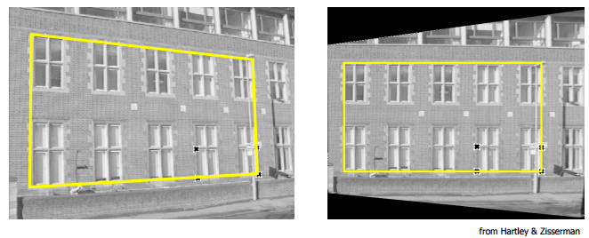
由两个相机位置观察到的平面（图像摘自 3 和 2）

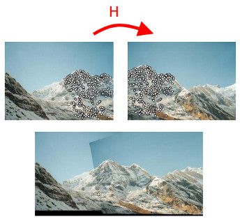
相机绕其投影轴旋转，等效于认为点位于无穷远平面上（图像摘自 2）

单应变换有何用处？

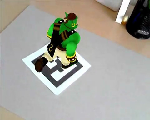
例如，通过标记从共面点进行增强现实中的相机位姿估计（参见前面的第一个示例）

透视消除/校正（参见前面的第二个示例）

全景图像拼接（参见前面的第二个和第三个示例）

演示代码

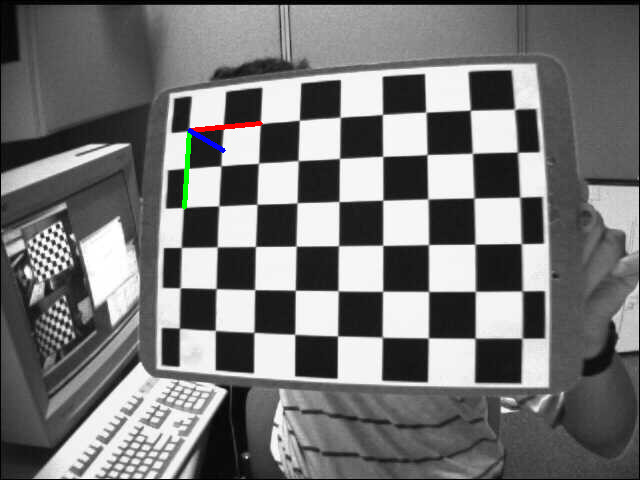
演示1：从共面点进行位姿估计

注意: 请注意，从单应性估计相机位姿的代码只是一个示例，如果您想估计平面或任意物体的相机位姿，应该使用 cv::solvePnP。

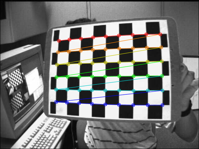
单应性可以使用例如直接线性变换（DLT）算法进行估计（更多信息请参见 1）。由于物体是平面的，因此在物体坐标系中表示的点与在归一化相机坐标系中表示的投影到图像平面上的点之间的变换是单应性。仅当物体是平面时，才能从单应性中恢复相机位姿，前提是相机内参已知（参见 2 或 4）。这可以通过使用棋盘格物体和 findChessboardCorners() 函数轻松测试，以获取图像中的角点位置。

首先是检测棋盘格角点，需要棋盘格大小（patternSize），这里是 9x6

vector<Point2f> corners;

bool found = findChessboardCorners(img, patternSize, corners);

已知棋盘格方块的大小，可以轻松计算在物体坐标系中表示的物体点

        for( int i = 0; i < boardSize.height; i++ )
            for( int j = 0; j < boardSize.width; j++ )
corners.push_back(Point3f(float(j*squareSize),
                                          float(i*squareSize), 0));

在单应性估计部分必须移除 Z=0 坐标

vector<Point3f> objectPoints;
calcChessboardCorners(patternSize, squareSize, objectPoints);
vector<Point2f> objectPointsPlanar;
    for (size_t i = 0; i < objectPoints.size(); i++)
    {
objectPointsPlanar.push_back(Point2f(objectPoints[i].x, objectPoints[i].y));
    }

归一化相机中的图像点可以通过角点并应用使用相机内参和畸变系数的反透视变换来计算

    FileStorage fs( samples::findFile( intrinsicsPath ), FileStorage::READ);
    Mat cameraMatrix, distCoeffs;
fs["camera_matrix"] >> cameraMatrix;
fs["distortion_coefficients"] >> distCoeffs;

vector<Point2f> imagePoints;

undistortPoints(corners, imagePoints, cameraMatrix, distCoeffs);

然后可以使用以下方法估计单应性

Mat H = findHomography(objectPointsPlanar, imagePoints);

cout << "H:\n" << H << endl;

从单应矩阵中检索位姿的快速解决方案是（参见 5）

    // Normalization to ensure that ||c1|| = 1
    double norm = sqrt(H.at<double>(0,0)*H.at<double>(0,0) +
H.at<double>(1,0)*H.at<double>(1,0) +
H.at<double>(2,0)*H.at<double>(2,0));
 
H /= norm;
    Mat c1 = H.col(0);
    Mat c2 = H.col(1);
    Mat c3 = c1.cross(c2);
 
    Mat tvec = H.col(2);
    Mat R(3, 3, CV_64F);
 
    for (int i = 0; i < 3; i++)
    {
R.at<double>(i,0) = c1.at<double>(i,0);
R.at<double>(i,1) = c2.at<double>(i,0);
R.at<double>(i,2) = c3.at<double>(i,0);
    }

\[ \begin{align*} \mathbf{X} &= \left( X, Y, 0, 1 \right ) \\ \mathbf{x} &= \mathbf{P}\mathbf{X} \\ &= \mathbf{K} \left[ \mathbf{r_1} \hspace{0.5em} \mathbf{r_2} \hspace{0.5em} \mathbf{r_3} \hspace{0.5em} \mathbf{t} \right ] \begin{pmatrix} X \\ Y \\ 0 \\ 1 \end{pmatrix} \\ &= \mathbf{K} \left[ \mathbf{r_1} \hspace{0.5em} \mathbf{r_2} \hspace{0.5em} \mathbf{t} \right ] \begin{pmatrix} X \\ Y \\ 1 \end{pmatrix} \\ &= \mathbf{H} \begin{pmatrix} X \\ Y \\ 1 \end{pmatrix} \end{align*} \]

\[ \begin{align*} \mathbf{H} &= \lambda \mathbf{K} \left[ \mathbf{r_1} \hspace{0.5em} \mathbf{r_2} \hspace{0.5em} \mathbf{t} \right ] \\ \mathbf{K}^{-1} \mathbf{H} &= \lambda \left[ \mathbf{r_1} \hspace{0.5em} \mathbf{r_2} \hspace{0.5em} \mathbf{t} \right ] \\ \mathbf{P} &= \mathbf{K} \left[ \mathbf{r_1} \hspace{0.5em} \mathbf{r_2} \hspace{0.5em} \left( \mathbf{r_1} \times \mathbf{r_2} \right ) \hspace{0.5em} \mathbf{t} \right ] \end{align*} \]

这是一个快速解决方案（另见 2），因为它不能确保结果旋转矩阵是正交的，并且尺度通过将第一列归一化为 1 来粗略估计。

获得一个适当的旋转矩阵（具有旋转矩阵的特性）的解决方案是应用极分解，或对旋转矩阵进行正交化（有关信息请参见 6 或 7 或 8 或 9）

cout << "R (before polar decomposition):\n" << R << "\ndet(R): " << determinant(R) << endl;
    Mat_<double> W, U, Vt;
    SVDecomp(R, W, U, Vt);
R = U*Vt;
    double det = determinant(R);
    if (det < 0)
    {
Vt.at<double>(2,0) *= -1;
Vt.at<double>(2,1) *= -1;
Vt.at<double>(2,2) *= -1;
 
R = U*Vt;
    }
cout << "R (after polar decomposition):\n" << R << "\ndet(R): " << determinant(R) << endl;

为检查结果，显示了使用估计的相机位姿投影到图像中的物体坐标系

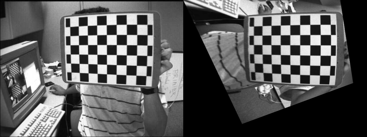
演示2：透视校正

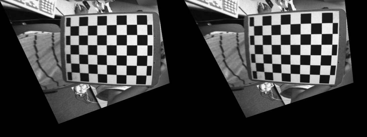
在此示例中，通过计算将源点映射到目标点的单应性，将源图像转换为所需的透视视图。下图显示了源图像（左）和我们想要转换为目标棋盘视图的棋盘视图（右）。

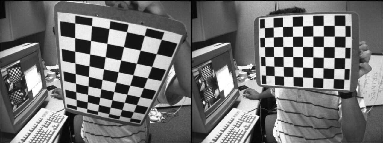
源视图和目标视图

第一步是在源图像和目标图像中检测棋盘格角点

单应性可以轻松估计

为了将源棋盘视图扭曲到目标棋盘视图，我们使用 cv::warpPerspective

结果图像是

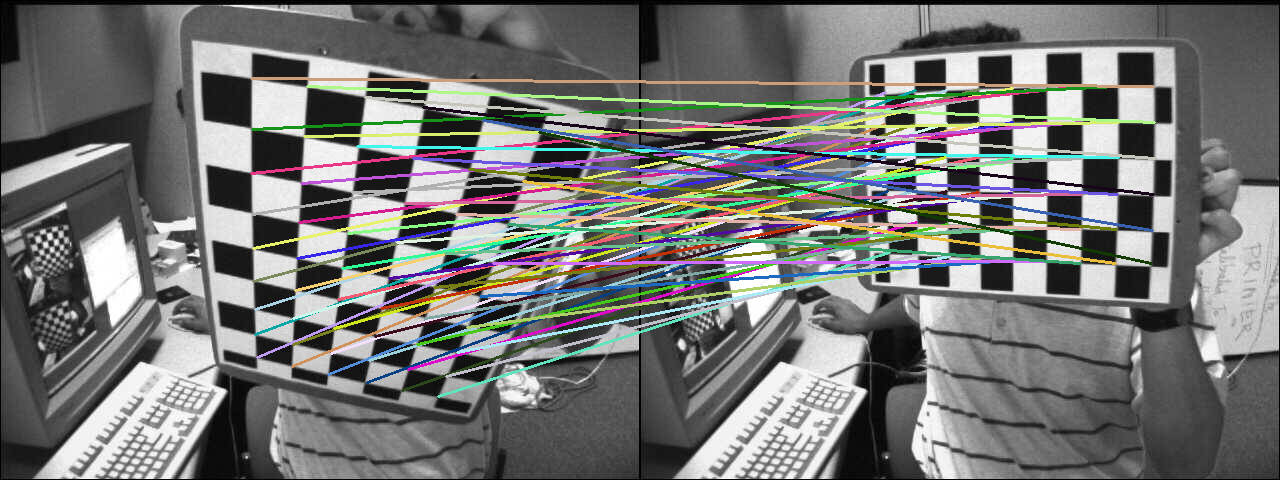
计算通过单应性变换的源角点坐标

为了检查计算的正确性，显示了匹配线

演示3：从相机位移计算单应

单应性关联了两个平面之间的变换，并且可以检索相应的相机位移，该位移允许从第一个平面视图转换到第二个平面视图（更多信息请参见 [183]）。在深入探讨如何从相机位移计算单应性的细节之前，先回顾一下相机位姿和齐次变换。

函数 cv::solvePnP 允许从对应的 3D 物体点（在物体坐标系中表示的点）和投影的 2D 图像点（在图像中观察到的物体点）计算相机位姿。需要内参和畸变系数（参见相机标定过程）。

\[ \begin{align*} s \begin{bmatrix} u \\ v \\ 1 \end{bmatrix} &= \begin{bmatrix} f_x & 0 & c_x \\ 0 & f_y & c_y \\ 0 & 0 & 1 \end{bmatrix} \begin{bmatrix} r_{11} & r_{12} & r_{13} & t_x \\ r_{21} & r_{22} & r_{23} & t_y \\ r_{31} & r_{32} & r_{33} & t_z \end{bmatrix} \begin{bmatrix} X_o \\ Y_o \\ Z_o \\ 1 \end{bmatrix} \\ &= \mathbf{K} \hspace{0.2em} ^{c}\mathbf{M}_o \begin{bmatrix} X_o \\ Y_o \\ Z_o \\ 1 \end{bmatrix} \end{align*} \]

\( \mathbf{K} \) 是内参矩阵，\( ^{c}\mathbf{M}_o \) 是相机位姿。cv::solvePnP 的输出正是如此：rvec 是罗德里格斯旋转向量，tvec 是平移向量。

\( ^{c}\mathbf{M}_o \) 可以用齐次形式表示，并允许将物体坐标系中表示的点变换到相机坐标系中

\[ \begin{align*} \begin{bmatrix} X_c \\ Y_c \\ Z_c \\ 1 \end{bmatrix} &= \hspace{0.2em} ^{c}\mathbf{M}_o \begin{bmatrix} X_o \\ Y_o \\ Z_o \\ 1 \end{bmatrix} \\ &= \begin{bmatrix} ^{c}\mathbf{R}_o & ^{c}\mathbf{t}_o \\ 0_{1\times3} & 1 \end{bmatrix} \begin{bmatrix} X_o \\ Y_o \\ Z_o \\ 1 \end{bmatrix} \\ &= \begin{bmatrix} r_{11} & r_{12} & r_{13} & t_x \\ r_{21} & r_{22} & r_{23} & t_y \\ r_{31} & r_{32} & r_{33} & t_z \\ 0 & 0 & 0 & 1 \end{bmatrix} \begin{bmatrix} X_o \\ Y_o \\ Z_o \\ 1 \end{bmatrix} \end{align*} \]

将一个坐标系中表示的点变换到另一个坐标系中可以很容易地通过矩阵乘法完成

\( ^{c_1}\mathbf{M}_o \) 是相机 1 的相机位姿
\( ^{c_2}\mathbf{M}_o \) 是相机 2 的相机位姿

要将相机 1 坐标系中表示的 3D 点变换到相机 2 坐标系中

\[ ^{c_2}\mathbf{M}_{c_1} = \hspace{0.2em} ^{c_2}\mathbf{M}_{o} \cdot \hspace{0.1em} ^{o}\mathbf{M}_{c_1} = \hspace{0.2em} ^{c_2}\mathbf{M}_{o} \cdot \hspace{0.1em} \left( ^{c_1}\mathbf{M}_{o} \right )^{-1} = \begin{bmatrix} ^{c_2}\mathbf{R}_{o} & ^{c_2}\mathbf{t}_{o} \\ 0_{3 \times 1} & 1 \end{bmatrix} \cdot \begin{bmatrix} ^{c_1}\mathbf{R}_{o}^T & - \hspace{0.2em} ^{c_1}\mathbf{R}_{o}^T \cdot \hspace{0.2em} ^{c_1}\mathbf{t}_{o} \\ 0_{1 \times 3} & 1 \end{bmatrix} \]

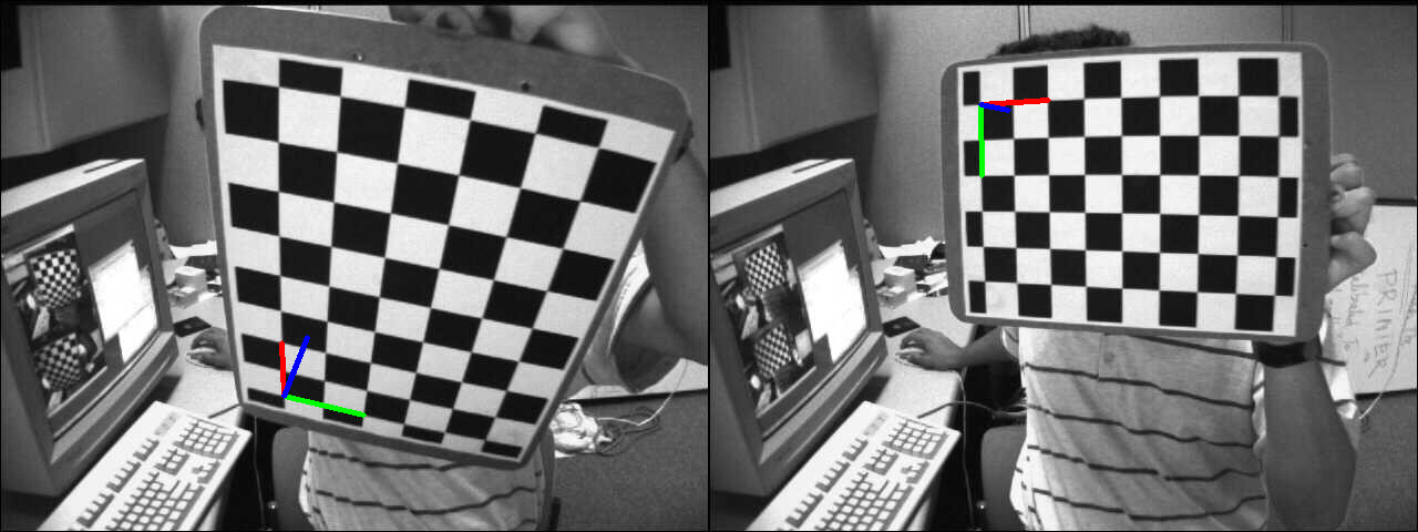
在此示例中，我们将计算相对于棋盘格物体，两个相机位姿之间的相机位移。第一步是计算两幅图像的相机位姿

vector<Point2f> corners1, corners2;
    bool found1 = findChessboardCorners(img1, patternSize, corners1);
    bool found2 = findChessboardCorners(img2, patternSize, corners2);
 
    if (!found1 || !found2)
    {
cout << "Error, cannot find the chessboard corners in both images." << endl;
        return;
    }
 
vector<Point3f> objectPoints;
calcChessboardCorners(patternSize, squareSize, objectPoints);
 
    FileStorage fs( samples::findFile( intrinsicsPath ), FileStorage::READ);
    Mat cameraMatrix, distCoeffs;
fs["camera_matrix"] >> cameraMatrix;
fs["distortion_coefficients"] >> distCoeffs;
 
    Mat rvec1, tvec1;
    solvePnP(objectPoints, corners1, cameraMatrix, distCoeffs, rvec1, tvec1);
    Mat rvec2, tvec2;
    solvePnP(objectPoints, corners2, cameraMatrix, distCoeffs, rvec2, tvec2);

相机位移可以使用上述公式从相机位姿计算得出

void computeC2MC1(const Mat &R1, const Mat &tvec1, const Mat &R2, const Mat &tvec2,
                  Mat &R_1to2, Mat &tvec_1to2)
{
    //c2Mc1 = c2Mo * oMc1 = c2Mo * c1Mo.inv()
R_1to2 = R2 * R1.t();
tvec_1to2 = R2 * (-R1.t()*tvec1) + tvec2;
}

从相机位移计算出的与特定平面相关的单应性是

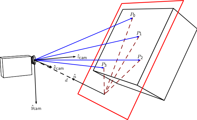
图片来源：Homography-transl.svg：Per Rosengren 衍生作品：Appoose (Homography-transl.svg) [CC BY 3.0 (http://creativecommons.org/licenses/by/3.0)]，通过维基共享资源

在此图中，n 是平面的法向量，d 是相机坐标系与平面沿平面法线方向的距离。从相机位移计算单应性的方程是

\[ ^{2}\mathbf{H}_{1} = \hspace{0.2em} ^{2}\mathbf{R}_{1} - \hspace{0.1em} \frac{^{2}\mathbf{t}_{1} \cdot \hspace{0.1em} ^{1}\mathbf{n}^\top}{^1d} \]

其中 \( ^{2}\mathbf{H}_{1} \) 是将第一个相机坐标系中的点映射到第二个相机坐标系中对应点的单应矩阵，\( ^{2}\mathbf{R}_{1} = \hspace{0.2em} ^{c_2}\mathbf{R}_{o} \cdot \hspace{0.1em} ^{c_1}\mathbf{R}_{o}^{\top} \) 是表示两个相机坐标系之间旋转的旋转矩阵，而 \( ^{2}\mathbf{t}_{1} = \hspace{0.2em} ^{c_2}\mathbf{R}_{o} \cdot \left( - \hspace{0.1em} ^{c_1}\mathbf{R}_{o}^{\top} \cdot \hspace{0.1em} ^{c_1}\mathbf{t}_{o} \right ) + \hspace{0.1em} ^{c_2}\mathbf{t}_{o} \) 是两个相机坐标系之间的平移向量。

这里的法向量 n 是在相机坐标系 1 中表示的平面法线，可以计算为 2 个向量的叉积（使用平面上的 3 个不共线点），或者在我们的例子中直接使用

Mat normal = (Mat_<double>(3,1) << 0, 0, 1);

Mat normal1 = R1*normal;

距离 d 可以计算为平面法线与平面上一点的点积，或者通过计算平面方程并使用 D 系数

    Mat origin(3, 1, CV_64F, Scalar(0));
    Mat origin1 = R1*origin + tvec1;
    double d_inv1 = 1.0 / normal1.dot(origin1);

投影单应矩阵 \( \textbf{G} \) 可以使用内参矩阵 \( \textbf{K} \) 从欧几里得单应性 \( \textbf{H} \) 计算得出（参见 [183]），这里假设两个平面视图之间使用相同的相机

\[ \textbf{G} = \gamma \textbf{K} \textbf{H} \textbf{K}^{-1} \]

Mat computeHomography(const Mat &R_1to2, const Mat &tvec_1to2, const double d_inv, const Mat &normal)
{
    Mat homography = R_1to2 + d_inv * tvec_1to2*normal.t();
    return homography;
}

在我们的例子中，棋盘格的 Z 轴指向物体内部，而在单应图例中它指向外部。这只是一个符号问题

\[ ^{2}\mathbf{H}_{1} = \hspace{0.2em} ^{2}\mathbf{R}_{1} + \hspace{0.1em} \frac{^{2}\mathbf{t}_{1} \cdot \hspace{0.1em} ^{1}\mathbf{n}^\top}{^1d} \]

    Mat homography_euclidean = computeHomography(R_1to2, t_1to2, d_inv1, normal1);
    Mat homography = cameraMatrix * homography_euclidean * cameraMatrix.inv();
 
homography /= homography.at<double>(2,2);
homography_euclidean /= homography_euclidean.at<double>(2,2);

我们现在将比较从相机位移计算的投影单应性与使用 cv::findHomography 估计的单应性。

findHomography H
[0.32903393332201, -1.244138808862929, 536.4769088231476;
 0.6969763913334046, -0.08935909072571542, -80.34068504082403;
 0.00040511729592961, -0.001079740100565013, 0.9999999999999999]
 
从相机位移计算的单应性
[0.4160569997384721, -1.306889006892538, 553.7055461075881;
 0.7917584252773352, -0.06341244158456338, -108.2770029401219;
 0.0005926357240956578, -0.001020651672127799, 1]

单应矩阵相似。如果我们比较使用两个单应矩阵扭曲的图像 1

左：使用估计单应性扭曲的图像。右：使用从相机位移计算的单应性。

从视觉上看，很难区分从相机位移计算的单应性与使用 cv::findHomography 函数估计的单应性所产生的图像差异。

练习

这个演示展示了如何从两个相机位姿计算单应变换。尝试执行相同的操作，但这次计算 N 个中间单应性。不要计算一个单应性直接将源图像扭曲到所需的相机视点，而是执行 N 次扭曲操作以查看不同的变换效果。

您应该得到类似以下的结果

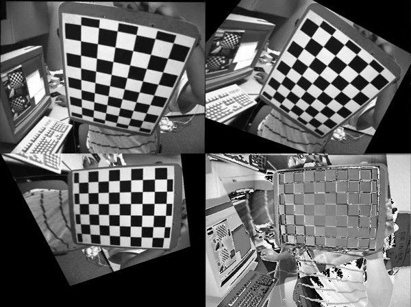
前三幅图像显示了源图像在三个不同的插值相机视点处被扭曲。第四幅图像显示了在最终相机视点处扭曲的源图像与目标图像之间的“误差图像”。

演示4：分解单应矩阵

OpenCV 3 包含了函数 cv::decomposeHomographyMat，它允许将单应矩阵分解为一组旋转、平移和平面法线。首先，我们将分解从相机位移计算的单应矩阵

    Mat homography_euclidean = computeHomography(R_1to2, t_1to2, d_inv1, normal1);
    Mat homography = cameraMatrix * homography_euclidean * cameraMatrix.inv();
 
homography /= homography.at<double>(2,2);
homography_euclidean /= homography_euclidean.at<double>(2,2);

cv::decomposeHomographyMat 的结果是

vector<Mat> Rs_decomp, ts_decomp, normals_decomp;
    int solutions = decomposeHomographyMat(homography, cameraMatrix, Rs_decomp, ts_decomp, normals_decomp);
cout << "Decompose homography matrix computed from the camera displacement:" << endl << endl;
    for (int i = 0; i < solutions; i++)
    {
      double factor_d1 = 1.0 / d_inv1;
      Mat rvec_decomp;
      Rodrigues(Rs_decomp[i], rvec_decomp);
cout << "Solution " << i << ":" << endl;
cout << "rvec from homography decomposition: " << rvec_decomp.t() << endl;
cout << "rvec from camera displacement: " << rvec_1to2.t() << endl;
cout << "tvec from homography decomposition: " << ts_decomp[i].t() << " and scaled by d: " << factor_d1 * ts_decomp[i].t() << endl;
cout << "tvec from camera displacement: " << t_1to2.t() << endl;
cout << "plane normal from homography decomposition: " << normals_decomp[i].t() << endl;
cout << "plane normal at camera 1 pose: " << normal1.t() << endl << endl;
    }

Solution 0
rvec from homography decomposition: [-0.0919829920641369, -0.5372581036567992, 1.310868863540717]
rvec from camera displacement: [-0.09198299206413783, -0.5372581036567995, 1.310868863540717]
tvec from homography decomposition: [-0.7747961019053186, -0.02751124463434032, -0.6791980037590677] and scaled by d: [-0.1578091561210742, -0.005603443652993778, -0.1383378976078466]
tvec from camera displacement: [0.1578091561210745, 0.005603443652993617, 0.1383378976078466]
plane normal from homography decomposition: [-0.1973513139420648, 0.6283451996579074, -0.7524857267431757]
plane normal at camera 1 pose: [0.1973513139420654, -0.6283451996579068, 0.752485726743176]
 
Solution 1
rvec from homography decomposition: [-0.0919829920641369, -0.5372581036567992, 1.310868863540717]
rvec from camera displacement: [-0.09198299206413783, -0.5372581036567995, 1.310868863540717]
tvec from homography decomposition: [0.7747961019053186, 0.02751124463434032, 0.6791980037590677] and scaled by d: [0.1578091561210742, 0.005603443652993778, 0.1383378976078466]
tvec from camera displacement: [0.1578091561210745, 0.005603443652993617, 0.1383378976078466]
plane normal from homography decomposition: [0.1973513139420648, -0.6283451996579074, 0.7524857267431757]
plane normal at camera 1 pose: [0.1973513139420654, -0.6283451996579068, 0.752485726743176]
 
Solution 2
rvec from homography decomposition: [0.1053487907109967, -0.1561929144786397, 1.401356552358475]
rvec from camera displacement: [-0.09198299206413783, -0.5372581036567995, 1.310868863540717]
tvec from homography decomposition: [-0.4666552552894618, 0.1050032934770042, -0.913007654671646] and scaled by d: [-0.0950475510338766, 0.02138689274867372, -0.1859598508065552]
tvec from camera displacement: [0.1578091561210745, 0.005603443652993617, 0.1383378976078466]
plane normal from homography decomposition: [-0.3131715472900788, 0.8421206145721947, -0.4390403768225507]
plane normal at camera 1 pose: [0.1973513139420654, -0.6283451996579068, 0.752485726743176]
 
Solution 3
rvec from homography decomposition: [0.1053487907109967, -0.1561929144786397, 1.401356552358475]
rvec from camera displacement: [-0.09198299206413783, -0.5372581036567995, 1.310868863540717]
tvec from homography decomposition: [0.4666552552894618, -0.1050032934770042, 0.913007654671646] and scaled by d: [0.0950475510338766, -0.02138689274867372, 0.1859598508065552]
tvec from camera displacement: [0.1578091561210745, 0.005603443652993617, 0.1383378976078466]
plane normal from homography decomposition: [0.3131715472900788, -0.8421206145721947, 0.4390403768225507]
plane normal at camera 1 pose: [0.1973513139420654, -0.6283451996579068, 0.752485726743176]

单应矩阵分解的结果只能恢复到一个尺度因子，该尺度因子实际上对应于距离 d，因为法线是单位长度。正如您所看到的，有一个解决方案与计算出的相机位移几乎完美匹配。正如文档中所述

如果通过应用正深度约束（所有点必须在相机前面）可获得点对应关系，则至少两个解可能会进一步失效。

由于分解结果是相机位移，如果我们有初始相机位姿 \( ^{c_1}\mathbf{M}_{o} \)，我们可以计算当前相机位姿 \( ^{c_2}\mathbf{M}_{o} = \hspace{0.2em} ^{c_2}\mathbf{M}_{c_1} \cdot \hspace{0.1em} ^{c_1}\mathbf{M}_{o} \)，并测试属于该平面的 3D 物体点是否投影到相机前方。另一种解决方案是，如果我们知道在相机 1 位姿下表示的平面法线，则保留具有最接近法线的解决方案。

同样的操作，但使用 cv::findHomography 估计的单应矩阵

Solution 0
rvec from homography decomposition: [0.1552207729599141, -0.152132696119647, 1.323678695078694]
rvec from camera displacement: [-0.09198299206413783, -0.5372581036567995, 1.310868863540717]
tvec from homography decomposition: [-0.4482361704818117, 0.02485247635491922, -1.034409687207331] and scaled by d: [-0.09129598307571339, 0.005061910238634657, -0.2106868109173855]
tvec from camera displacement: [0.1578091561210745, 0.005603443652993617, 0.1383378976078466]
plane normal from homography decomposition: [-0.1384902722707529, 0.9063331452766947, -0.3992250922214516]
plane normal at camera 1 pose: [0.1973513139420654, -0.6283451996579068, 0.752485726743176]
 
Solution 1
rvec from homography decomposition: [0.1552207729599141, -0.152132696119647, 1.323678695078694]
rvec from camera displacement: [-0.09198299206413783, -0.5372581036567995, 1.310868863540717]
tvec from homography decomposition: [0.4482361704818117, -0.02485247635491922, 1.034409687207331] and scaled by d: [0.09129598307571339, -0.005061910238634657, 0.2106868109173855]
tvec from camera displacement: [0.1578091561210745, 0.005603443652993617, 0.1383378976078466]
plane normal from homography decomposition: [0.1384902722707529, -0.9063331452766947, 0.3992250922214516]
plane normal at camera 1 pose: [0.1973513139420654, -0.6283451996579068, 0.752485726743176]
 
Solution 2
rvec from homography decomposition: [-0.2886605671759886, -0.521049903923871, 1.381242030882511]
rvec from camera displacement: [-0.09198299206413783, -0.5372581036567995, 1.310868863540717]
tvec from homography decomposition: [-0.8705961357284295, 0.1353018038908477, -0.7037702049789747] and scaled by d: [-0.177321544550518, 0.02755804196893467, -0.1433427218822783]
tvec from camera displacement: [0.1578091561210745, 0.005603443652993617, 0.1383378976078466]
plane normal from homography decomposition: [-0.2284582117722427, 0.6009247303964522, -0.7659610393954643]
plane normal at camera 1 pose: [0.1973513139420654, -0.6283451996579068, 0.752485726743176]
 
Solution 3
rvec from homography decomposition: [-0.2886605671759886, -0.521049903923871, 1.381242030882511]
rvec from camera displacement: [-0.09198299206413783, -0.5372581036567995, 1.310868863540717]
tvec from homography decomposition: [0.8705961357284295, -0.1353018038908477, 0.7037702049789747] and scaled by d: [0.177321544550518, -0.02755804196893467, 0.1433427218822783]
tvec from camera displacement: [0.1578091561210745, 0.005603443652993617, 0.1383378976078466]
plane normal from homography decomposition: [0.2284582117722427, -0.6009247303964522, 0.7659610393954643]
plane normal at camera 1 pose: [0.1973513139420654, -0.6283451996579068, 0.752485726743176]

同样，也存在与计算出的相机位移匹配的解。

演示5：基于旋转相机的基本全景图像拼接

注意: 此示例旨在说明基于相机纯旋转运动的图像拼接概念，不应直接用于拼接全景图像。拼接模块提供了完整的图像拼接流程。

单应变换仅适用于平面结构。但在相机旋转（纯粹绕相机投影轴旋转，无平移）的情况下，可以考虑任意世界（参见前文）。

然后可以使用旋转变换和相机内参计算单应性，公式如下（例如参见 10）

\[ s \begin{bmatrix} x^{'} \\ y^{'} \\ 1 \end{bmatrix} = \bf{K} \hspace{0.1em} \bf{R} \hspace{0.1em} \bf{K}^{-1} \begin{bmatrix} x \\ y \\ 1 \end{bmatrix} \]

为了说明这一点，我们使用了 Blender（一款免费开源的 3D 计算机图形软件）来生成两个相机视图，它们之间只有旋转变换。有关如何使用 Blender 获取相机内参和相对于世界的 3x4 外参矩阵的更多信息，请参见 11（还需要一个额外的变换才能获得相机与物体坐标系之间的变换）。

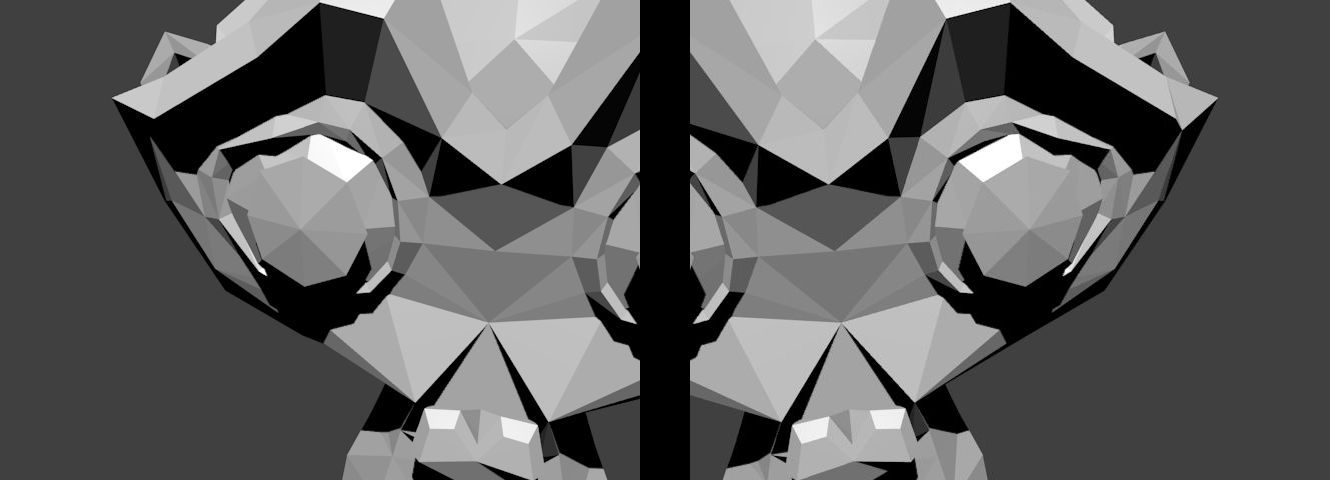
下图显示了 Suzanne 模型生成的两个视图，它们之间只有旋转变换

已知关联的相机位姿和内参，可以计算两个视图之间的相对旋转

这里，第二幅图像将相对于第一幅图像进行拼接。单应性可以使用上述公式计算

拼接操作很简单